
ミーンシフトの計算例を載せます。
import numpy as np
import matplotlib.pyplot as plt
import cv2
#from mpl_toolkits.mplot3d import Axes3D

rgb_img = plt.imread('c:/temp/test.bmp')

#plt.imread こちらはBGRの順で扱う
#cv2.imread こちらはRGBの順で扱う

#もし変換したかったらこちらを使う
#rgb_img = cv2.cvtColor(rgb_img, cv2.COLOR_BGR2RGB)

fig = plt.figure(figsize=(10, 5))
plt.subplot(1, 2, 1)
plt.imshow(rgb_img)

plt.subplot(1, 2, 2)
ax = fig.add_subplot(122, projection='3d')
ax.scatter3D(rgb_img[:,:,0], rgb_img[:,:,1], rgb_img[:,:,2])

ax.set_xlabel('R_axis')
ax.set_ylabel('G_axis')
ax.set_zlabel('B axis')

plt.show()
print("finishi")
import numpy as np
import matplotlib.pyplot as plt
import cv2
import pandas as pd
import matplotlib.cm as cm

from sklearn import cluster
from sklearn.cluster import MeanShift,estimate_bandwidth
import warnings
warnings.simplefilter('ignore', FutureWarning)

#from mpl_toolkits.mplot3d import Axes3D

rgb_img = plt.imread('c:/temp/test.bmp')

rgb0 = rgb_img[:,:,0]
rgb1 = rgb_img[:,:,1]
rgb2 = rgb_img[:,:,2]
x1 = range(0,rgb_img.shape[1])
x2 = range(0,rgb_img.shape[0])
x1, x2 = np.meshgrid(x1,x2)

rgb = np.array([rgb0, rgb1, rgb2, x1, x2]).reshape(5,rgb_img.shape[0]*rgb_img.shape[1])
df = pd.DataFrame(rgb.T)
df.columns = ['red', 'green', 'blue', 'x1', 'x2']
df.head()

# k-means
km=cluster.KMeans(n_clusters=10)
z_km=km.fit(df)

# MeanShift
bwidth = estimate_bandwidth(df.values,quantile=0.15,n_samples=200)
ms = cluster.MeanShift(seeds=df.values, bandwidth=bwidth)
ms.fit(df.values)


fig, ax = plt.subplots(1, 2, figsize=(10, 4))

ax[0].scatter(df["red"], df["blue"], c=cm.hsv(ms.labels_/len(ms.cluster_centers_)))
ax[0].scatter(ms.cluster_centers_[:,0], ms.cluster_centers_[:,2],s=250, marker='*',c='orange')
ax[0].set_title("Mean Shift");

ax[1].scatter(df["red"], df["blue"], c=cm.hsv(z_km.labels_/len(z_km.cluster_centers_)))
ax[1].scatter(z_km.cluster_centers_[:,0],z_km.cluster_centers_[:,2],s=250, marker='*',c='orange')
ax[1].set_title("k-means");

plt.show()
print("finishi")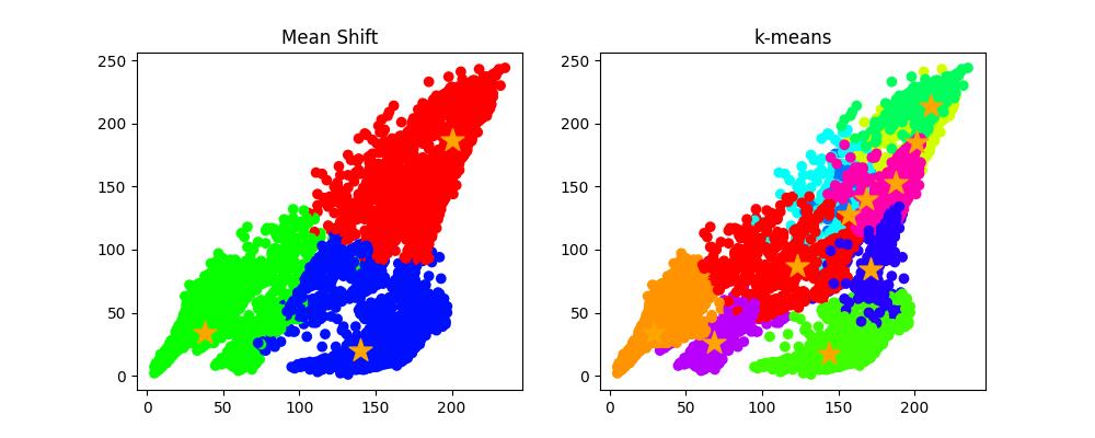
import numpy as np
import matplotlib.pyplot as plt
import cv2
import pandas as pd
import matplotlib.cm as cm

from sklearn import cluster
from sklearn.cluster import MeanShift,estimate_bandwidth
import warnings
warnings.simplefilter('ignore', FutureWarning)

#from mpl_toolkits.mplot3d import Axes3D

rgb_img = plt.imread('c:/temp/test.bmp')

rgb0 = rgb_img[:,:,0]
rgb1 = rgb_img[:,:,1]
rgb2 = rgb_img[:,:,2]
x1 = range(0,rgb_img.shape[1])
x2 = range(0,rgb_img.shape[0])
x1, x2 = np.meshgrid(x1,x2)

rgb = np.array([rgb0, rgb1, rgb2, x1, x2]).reshape(5,rgb_img.shape[0]*rgb_img.shape[1])
df = pd.DataFrame(rgb.T)
df.columns = ['red', 'green', 'blue', 'x1', 'x2']
df.head()

# k-means
km=cluster.KMeans(n_clusters=10)
z_km=km.fit(df)

# MeanShift
bwidth = estimate_bandwidth(df.values,quantile=0.15,n_samples=200)
ms = cluster.MeanShift(seeds=df.values, bandwidth=bwidth)
ms.fit(df.values)


fig, ax = plt.subplots(1, 3, figsize=(20, 10), subplot_kw=({"xticks":(), "yticks":()}))

ax[0].imshow(rgb_img)
ax[1].imshow(ms.labels_.reshape(rgb_img.shape[0],rgb_img.shape[1]),cmap='hsv')
ax[1].set_title("Mean Shift");
ax[2].imshow(z_km.labels_.reshape(rgb_img.shape[0],rgb_img.shape[1]),cmap='hsv')
ax[2].set_title("k-means");

plt.show()
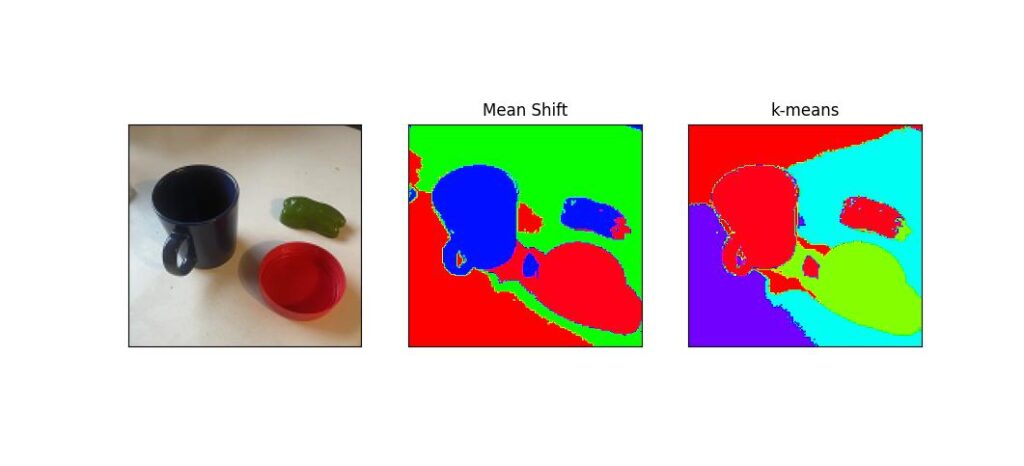
結構計算に時間がかかります。パラメータを変えると領域がいろいろ変わります。
 | ビジネスサイトを作って学ぶWordPressの教科書 Ver.5x対応版 [ プライム・ストラテジー ] 価格:3,080円 |
 | [改訂版]WordPress 仕事の現場でサッと使える! デザイン教科書[WordPress 5.x対応版] [ 中島真洋=著/ロクナナワークショップ=監修 ] 価格:3,058円 |


コメント